Real tropical geometry
silviana amethyst
2017
At some high level, for me Tropical Geometry is a relatively new (and arbitrarily named) field of mathematics studying the behaviour of algebraic varieties near coordinate hyperplane intersections. It’s also the study of the logarithmic transformation of \(\mathbb{C}\) algebra, as \(+\) maps to \(\max\), and as \(\times\) maps to \(+\). An absolutely fascinating topic.
My first foray into doing computations in Tropical Geometry came with the invitation to work with Jon Hauenstein and Cynthia Vinzant on the development of an algorithm to compute real tropical curves.
The resulting algorithm has been submitted to the Arxiv. Paper available here.
News 
I have written Matlab code calling Bertini 1 implementing the tropical curve decomposition algorithm Jon, Cynthia, and I developed. The code appears on the code page on this site under the curve section. The code is licensed using the GPL 3 license.
Some examples of using the code to compute tropical curves, both real and complex, are on the curve examples page.
Tropical curves 
Curves are dimension-one objects. One naturally expects curves to be present when the number of variables exceeds the number of equations or constraints by one, and when it does, we call this a complete intersection. When the intersection is complete, the number of equations is at least the number of variables. The twisted cubic is an example of such a curve – an incomplete intersection.
I have written Matlab code using Bertini to compute tropical curves. You can access it here.
There are some computed examples demonstrating the code in the examples page.
Code for computing tropical curves
I offer here a package of code implemented in Matlab for numerically decomposing tropical curves, as described in my joint paper with Jon Hauenstein and Cynthia Vinzant.
The code is offered under the GPL3 license for FLOSS.
Download the code here:
- bertini_tropical.zip (20170224)
The Matlab code offers several chunks of useful code, including
- a bertini_input_file class for Matlab, which is useful for constructing a system to solve using Bertini 1.x
- code for calling bertini, and doing some error checking
- a tropical_curve class for Matlab, which holds the rays coming from coordinate hyperplane intersections, and offers several useful functions for plotting and displaying the data
- code for actually performing the tropical curve decomposition, both for real and complex curves
Examples for how to use the code, particularly how to decompose real and complex tropical curves using Matlab and Bertini using your compute resources, is found in the examples section. Installation instructions, and basic usage instructions appear on separate pages.
Installing
There are only a few steps to install the code offered above. Briefly, they are
- Download and unpack the compressed folder to some memorable location. Let this location be $(P).
- Add $(P) to the path in Matlab. There is no need to add subfolders, as those are for the Matlab classes I wrote.
- Download and install Bertini. There’s a pre-compiled executable available, or you can compile from source.
- INSIDE MATLAB, add Bertini’s location to the path. This is NOT done via the regular path dialog box, but rather in some way similar to the one shown here.
- Test that you can run !bertini from within Matlab, without specifying a path. If not, goto 4.
- Download an md5 hasher for matlab, so you can call md5(file). I recommend one here. Ensure that md5 is on the path.
You should be good to go. I have prepared some brief running advice, and i have some worked examples, too.
If you have trouble, comments, or criticism, please write me an email.
Running
This assumes you have already installed the code, Bertini, and any necessary dependencies. If not, goto Installing.
- Create a folder in which to run some examples. Move there.
- Create a Bertini-style input file for your favorite curve. Start small, don’t go straight for that crazy 30-variable curve. How about one from the examples pages? Be sure to include the tracktype: 1; declaration in the config section, stating that you want a Numerical Irreducible Decomposition (NID). Also, you should homogenize and patch your system so you can compute the rays at \(\infty\). There are many examples of valid Bertini input files on the Bertini book page, though most are not curves.
- Call Bertini, compute the NID. Feel free to do this in parallel.
- If you did not get a dimension 1 component, stop, I cannot decompose higher dimension objects yet. Otherwise, keep going. The remainder of the steps must be in Matlab.
- Create a T=tropical_curve();, which by default is the complex curve. If you want the real part only, create T=tropical_curve(‘real’); The curve will automatically decompose.
- Since the software is numerical, there are thresholds which determine whether numbers are considered 0. If your results are not satisfactory, please consult the documentation, which should be included in the folder you downloaded.
Consider glancing over the examples.
If your results are still not satisfactory, you have challenges with the software, or have any comments or criticism, please contact me.
Examples
Parabola
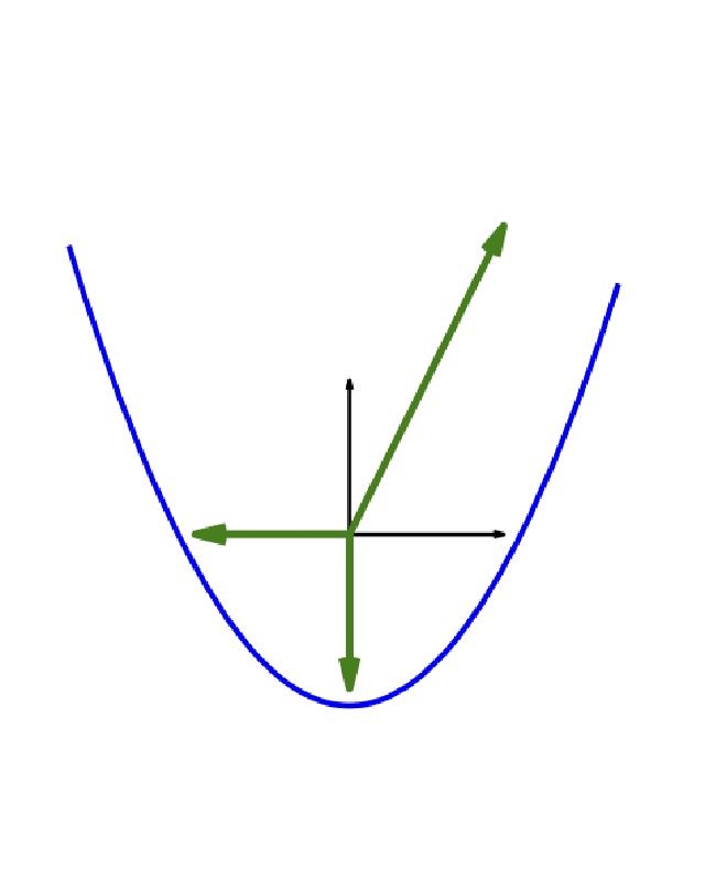
Setup
The first thing we’ll do is create a file containing the system describing the curve we want to decompose.
Since tropical geometric objects intersect the hyperplane at \(\infty\), we need to be able to compute points in this hyperplane. That’s right, we’ll compute points at \(\infty\)! The tool we’ll use is projectivization, a method of compactification which identifies all points on the same line as being the same point. This is accomplished by introducing a new variable to the system, called the homogenizing variable. We typically call it \(h\).
For our parabola, the starting system looks like
\[y = x^2-1,\]but we phrase problems in terms of a system vanishing, so we rewrite it as
\[ -y+ x^2-1=0.\]Now we homogenize. Every term (summand) in the system must have the same degree. The term \(y\) has degree 1, \(x^2\) has degree 2, and \(1\) has degree 0. The max is 2. Hence, each term needs to have degree 2. We increase degree by multiplying by the new homogenizing variable \(h\). Hence, the system becomes
\[h y + x^2 - h^2\]But now there are three variables and a single constraint, so it looks like a dimension-two object, whereas the parabola we started with was of dimension one.
The second part of projectivization is to introduce an affine patch. It picks out a single point on each line which is identified in projective space. We’ll choose a random patch,
\[p_h h + p_x x + p_y y -1 = 0.\]Finally we are ready to write the Bertini input file to be used to decompose the curve.
CONFIG

TrackType : 1;  %tell Bertini that we will be generating the NID for the system

END;

INPUT

variable_group h, x, y; %group variables into one group, in this order

function f1, patch;  %declarations

xsquared = x^2;
hsquared = h^2;  % not necessary, but demonstrating the code can use subfunctions.

f1 = xsquared - y*h - hsquared;

constant px, py, ph;  %there will be some constants

px = 0.052851867811043; %and here they are.
py = -0.729144193855660;
ph = -0.288589658032238;

patch = px*x + py*y + ph*h - 1;

END;
Note the top portion, bracketed by CONFIG and END;. Bertini 1 passes its configuration via a config section at the top of the input file. We will be working with positive-dimensional varieties, so we indicate to Bertini to generate a set of witness sets by passing tracktype: 1;.
Running
Now that we have our system set up in a Bertini input file, we will go through the steps to do the tropical decomposition.
NID
The input for the tropical decomposition includes the witness set for the component to be decomposed. Hence, we need ato generate that witness set. The Numerical Irreducible Decomposition (NID) contains that witness set, and the algorithm for computing it is accessed by using tracktype:1;.
All we need to do is call Bertini, assuming the input file is simply called ‘input’. Hence, move to the folder containing the input file (which you should name something corresponding to the system, such as ‘parabola’). This can be done either in a terminal, or in Matlab.
Then call Bertini. Let it run, for this system, it should complete very quickly, like less than one second. My output looks like this:
Bertini(TM) v1.5
  (February 11, 2015)

 D.J. Bates, J.D. Hauenstein,
 A.J. Sommese, C.W. Wampler

(using GMP v6.0.0, MPFR v3.1.3-p2)


NOTE: You have requested to use adaptive path tracking.  Please make sure that you have
setup the following tolerances appropriately:
CoeffBound: 2.133930000000e+00, DegreeBound: 2.000000000000e+00
AMPSafetyDigits1: 1, AMPSafetyDigits2: 1, AMPMaxPrec: 1024


Tracking regeneration codim 1 of 2: 2 paths to track.
Tracking path 0 of 2

Sorting codimension 1 of 2: 2 paths to sort.
Sorting 0 of 2

Preparing regeneration codim 2 of 2: 0 witness points to move.

Tracking regeneration codim 2 of 2: 2 paths to track.
Tracking path 0 of 2

Sorting codimension 2 of 2: 2 paths to sort.
Sorting 0 of 2


************ Regenerative Cascade Summary ************

NOTE: nonsingular vs singular is based on rank deficiency and identical endpoints

|codim|   paths   |witness superset| nonsingular | singular |nonsolutions| inf endpoints | other bad endpoints
----------------------------------------------------------------------------------------------------------------
| 1   |   2       |   0            |  0          |  0       |  2         |   0           |  0
| 2   |   2       |   2            |  2          |  0       |  0         |   0           |  0
----------------------------------------------------------------------------------------------------------------
|total|   4

****************************************************


*************** Witness Set Summary ****************

NOTE: nonsingular vs singular is based on rank deficiency and identical endpoints

|codim| witness points | nonsingular | singular
-------------------------------------------------
| 2   |   2            |  2          |  0
-------------------------------------------------

****************************************************


Calculating traces for codimension 2.
Calculating 0 of 2

Using combinatorial trace test to decompose codimension 2.


************* Witness Set Decomposition *************

| dimension | components | classified | unclassified
-----------------------------------------------------
|   1       |   1        |   2        |  0
-----------------------------------------------------

************** Decomposition by Degree **************

Dimension 1: 1 classified component
-----------------------------------------------------
   degree 2: 1 component

*****************************************************
The most important part is the last bit, where it tells us we have a single dimension 1 classified component, of degree 2. Briefly, this means that a random complex intersection with this component will yield two points. Indeed, the witness set contains two points.
The output from Bertini is the ‘witness data’ file, contained in the working folder.
Complex Tropical Decomposition - \(\mathbb{C}\)
Now that we have the NID in ‘witness_data’, we can compute the tropical decomposition of the component.
To do so, we simply create a ’tropical_curve’ object in Matlab. The constructor for this class, provided in this code, performs the decomposition. There are options you can pass in, such as whether you want the complex or real curve, and several numerical tolerances.
For now, let’s stick to default mode, which does the decomposition of the complex curve. Here’s what I get on my machine:
>> T = tropical_curve()
slicing h=0
slicing x=0
slicing y=0
preparing critical points input file
	setting up subfunctions in memory
	making functions in memory
	computing jacobian matrix
	computing partial derivatives of subfunctions
	doing partial derivative substitutions for detjac
	doing subfuncion substitutions for detjac
	doing substitutions for new subfunctions
regenerating to detjac function for generic critical points
done regenerating start solutions.
computing critical points for t = h
slicing value for t=h is 1.0000e-01
slicing near coordinate axis intersection
connecting slice points to intersection points
doing monodromy loops to determine unique paths
computing critical points for t = x
slicing value for t=x is 1.0000e-01
slicing near coordinate axis intersection
connecting slice points to intersection points
doing monodromy loops to determine unique paths
computing critical points for t = y
slicing value for t=y is 1.0000e-01
slicing near coordinate axis intersection
connecting slice points to intersection points
doing monodromy loops to determine unique paths
T =
  tropical_curve with properties:

                  is_real: 0
           is_homogenized: 1
    homogenizing_variable: 'h'
                     rays: [3x3 double]
           multiplicities: [1 1 2]
                variables: {3x1 cell}
             curve_system: {2x2 cell}
             subfunctions: {2x2 cell}
              system_name: 'parabola'
                 aux_data: [1x1 struct]
There’s a lot going on in that output. Beyond that, a folder has been made in the current directory, containing the data for the run, and the tropical curve you made was automatically saved to a time-stamped .mat file. I just got:
- a folder called parabola_complex_tropical_decomposition
- a file called tropdecomp_parabola_complex_1601261210.mat. The parabola part of these names is determined by the name of the working folder. The time stamp is evident.
The rays and multiplicities are the most important part of the tropical curve. If you look at the output, you can see that the object ‘T’ that we just made
- is not real
- is homogenized
- has some rays
- has some multiplicities
- and has a bunch of other data, including ‘aux_data’. To look at the rays, just call the name of the field in Matlab: ‘T.rays’.
>> T.rays
ans =
    -2     0     0
    -1    -1     0
     0     0    -1
One thing to notice is that there are too many coordinates in some sense. Well, we homogenized, first thing. We introduced a new variable, \(h\), and it appears at the front of the variable ordering. Let’s de-homogenize. I built the call into Matlab:
T.dehomogenize
ans =
  tropical_curve with properties:

                  is_real: 0
           is_homogenized: 0
    homogenizing_variable: 'h'
                     rays: [2x3 double]
           multiplicities: [1 1 2]
                variables: {'x'  'y'}
             curve_system: {2x2 cell}
             subfunctions: {2x2 cell}
              system_name: 'parabola'
                 aux_data: [1x1 struct]
Since tropical_curves are implemented as handle classes in Matlab, the call T.dehomogenize modifies T. It does not produce a new copy of T which is dehomogenized, but rather T itself changes. This is ok, the tropical curve automatically saved, so you can just re-load it from disk if you feel like you screwed something up.
Now let’s look at the rays, and their multiplicities, without the ’extra’ homogenizing variable mucking things up.
T.rays
ans =
     1    -1     0
     2     0    -1
>> T.multiplicities
ans =
     1     1     2
Sure enough, the rays are as expected. Columns in the matrix represent the rays. Ok, so we have rays and multiplicities, but do they balance? Ray-multiplicity structure balances for tropical curves, in the sense that they sum to 0, if you multiply each ray by its multiplicity, and add them all up for all rays, you should get 0. If not, then an error certainly occurred. Let’s check.
T.ray_sum
ans =
     0
     0
They balanced! The curve was decomposed correctly.
Real Tropical Decomposition - \(\mathbb{R}\)
We have successfully decomposed the parabola’s complex curve. What about what we usually think of as a parabola, the real curve? The code I provide can compute real tropicalizations, too! It starts from the point of a complete NID, just as the \(\mathbb{C}\) does. So we just call T = tropical_curve(‘real’) and let the algorithm go.
>> T = tropical_curve('real')
slicing h=0
slicing x=0
slicing y=0
preparing critical points input file
	setting up subfunctions in memory
	making functions in memory
	computing jacobian matrix
	computing partial derivatives of subfunctions
	doing partial derivative substitutions for detjac
	doing subfuncion substitutions for detjac
	doing substitutions for new subfunctions
regenerating to detjac function for generic critical points
done regenerating start solutions.
computing critical points for t = h
slicing value for t=h is 1.0000e-01
slicing near coordinate axis intersection
connecting slice points to intersection points
doing monodromy loops to determine unique paths
computing critical points for t = x
slicing value for t=x is 1.0000e-01
slicing near coordinate axis intersection
connecting slice points to intersection points
doing monodromy loops to determine unique paths
computing critical points for t = y
slicing value for t=y is 1.0000e-01
slicing near coordinate axis intersection
connecting slice points to intersection points
doing monodromy loops to determine unique paths
T =
  tropical_curve with properties:

                  is_real: 1
           is_homogenized: 1
    homogenizing_variable: 'h'
                     rays: [3x3 double]
           multiplicities: [1 1 2]
                variables: {3x1 cell}
             curve_system: {2x2 cell}
             subfunctions: {2x2 cell}
              system_name: 'parabola'
                 aux_data: [1x1 struct]
The data automatically saves, and the bread crumbs from the Bertini runs are preserved in their own folder, similarly to the complex case.
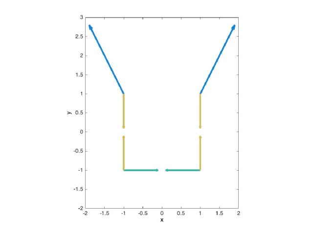
Real tropical curves can be arranged according to how the curve crosses the hyperplane, something which can’t be done for complex curves. The command ‘arrange’ for tropical real curves in Matlab will render the rays in space for me. First, let’s dehomogenize, then call arrange
>> T.dehomogenize
ans =
  tropical_curve with properties:

                  is_real: 1
           is_homogenized: 0
    homogenizing_variable: 'h'
                     rays: [2x3 double]
           multiplicities: [1 1 2]
                variables: {'x'  'y'}
             curve_system: {2x2 cell}
             subfunctions: {2x2 cell}
              system_name: 'parabola'
                 aux_data: [1x1 struct]
>> T.arrange
automatic text resizing available if command 'labelText' is installed
Ok, the code is letting me know that the command ’labelText’ will allow for re-sizing of the fonts in the image. Whatever. For now let’s just save it to disk, and put it here on this website.
print('parabola_arrangement','-djpeg')
Example: Quartic
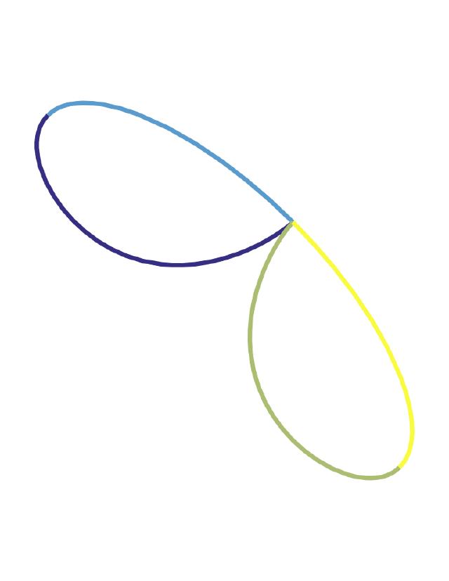
A quartic, which has some nice properties; e.g. it is compact, and it’s real tropicalization is not equal to the complex.
Setup
CONFIG

sharpendigits : 30;  %run Newton's method after tracking to get more digits

TrackType : 1;  %run the NID algorithm

END;

INPUT

variable_group h, x, y;

function f1, patch;

f1 = -(x-y)^2*(x+y)*h + x^4+y^4;  %the homogenized system we will solve

constant px, py, ph;

px = 0.052851867811043;
py = -0.729144193855660;
ph = -0.288589658032238;

patch = px*x + py*y + ph*h - 1; %its patch equation


END;
Running
NID Now that we have our system set up in a Bertini input file, we will go through the steps to do the tropical decomposition.
Then call Bertini 1.
>> !bertini

   Bertini(TM) v1.5
  (February 11, 2015)

 D.J. Bates, J.D. Hauenstein,
 A.J. Sommese, C.W. Wampler

(using GMP v6.0.0, MPFR v3.1.3-p2)


NOTE: You have requested to use adaptive path tracking.  Please make sure that you have
setup the following tolerances appropriately:
CoeffBound: 2.019082000000e+00, DegreeBound: 4.000000000000e+00
AMPSafetyDigits1: 1, AMPSafetyDigits2: 1, AMPMaxPrec: 1024


Tracking regeneration codim 1 of 2: 4 paths to track.
Tracking path 0 of 4

Sorting codimension 1 of 2: 4 paths to sort.
Sorting 0 of 4

Preparing regeneration codim 2 of 2: 0 witness points to move.

Tracking regeneration codim 2 of 2: 4 paths to track.
Tracking path 0 of 4

Sorting codimension 2 of 2: 4 paths to sort.
Sorting 0 of 4


************ Regenerative Cascade Summary ************

NOTE: nonsingular vs singular is based on rank deficiency and identical endpoints

|codim|   paths   |witness superset| nonsingular | singular |nonsolutions| inf endpoints | other bad endpoints
----------------------------------------------------------------------------------------------------------------
| 1   |   4       |   0            |  0          |  0       |  4         |   0           |  0
| 2   |   4       |   4            |  4          |  0       |  0         |   0           |  0
----------------------------------------------------------------------------------------------------------------
|total|   8

****************************************************


*************** Witness Set Summary ****************

NOTE: nonsingular vs singular is based on rank deficiency and identical endpoints

|codim| witness points | nonsingular | singular
-------------------------------------------------
| 2   |   4            |  4          |  0
-------------------------------------------------

****************************************************


Calculating traces for codimension 2.
Calculating 0 of 4

Using combinatorial trace test to decompose codimension 2.


************* Witness Set Decomposition *************

| dimension | components | classified | unclassified
-----------------------------------------------------
|   1       |   1        |   4        |  0
-----------------------------------------------------

************** Decomposition by Degree **************

Dimension 1: 1 classified component
-----------------------------------------------------
   degree 4: 1 component

*****************************************************
Bertini confirms a degree 4 dimension 1 component – the curve we will decompose.
Complex Tropical Decomposition - \(\mathbb{C}\)
Now that we have the NID in ‘witness_data’, we can compute the tropical decomposition of the component.
To do so, we simply create a ’tropical_curve’ object in Matlab. The constructor for this class, provided in this code, performs the decomposition. There are options you can pass in, such as whether you want the complex or real curve, and several numerical tolerances.
For now, let’s stick to default mode, which does the decomposition of the complex curve. Here’s what I get on my machine:
>> T = tropical_curve()
slicing h=0
slicing x=0
slicing y=0
preparing critical points input file
	setting up subfunctions in memory
	making functions in memory
	computing jacobian matrix
	computing partial derivatives of subfunctions
	doing partial derivative substitutions for detjac
	doing subfuncion substitutions for detjac
	doing substitutions for new subfunctions
regenerating to detjac function for generic critical points
done regenerating start solutions.
computing critical points for t = h
slicing value for t=h is 1.0000e-01
slicing near coordinate axis intersection
connecting slice points to intersection points
doing monodromy loops to determine unique paths
computing critical points for t = x
slicing value for t=x is 1.0000e-01
slicing near coordinate axis intersection
connecting slice points to intersection points
doing monodromy loops to determine unique paths
computing critical points for t = y
slicing value for t=y is 1.0000e-01
slicing near coordinate axis intersection
connecting slice points to intersection points
doing monodromy loops to determine unique paths
T =
  tropical_curve with properties:

                  is_real: 0
           is_homogenized: 1
    homogenizing_variable: 'h'
                     rays: [3x5 double]
           multiplicities: [4 1 1 1 1]
                variables: {3x1 cell}
             curve_system: {2x2 cell}
             subfunctions: {}
              system_name: 'crazyQuartic'
                 aux_data: [1x1 struct]
>> T.ray_sum
ans =
    -4
    -4
    -4
The curve decomposes on my system fairly rapidly, in about 5 seconds or less. The last command I run is T.ray_sum, checking the balancing condition for this decomposition. The weighted rays of a tropical curve balance to 0, but these balance to -4. What’s up with that?
The curve is still homogenized, which I did manually when preparing the system. So instead of balancing to 0, they sum to the negative of the degree of the component, in this case four. Dehomogenizing T and calling ray_sum properly balances.
Real Tropical Decomposition - \(\mathbb{R}\)
Now we will decompose the real part.
>> S = tropical_curve('real')
slicing h=0
slicing x=0
slicing y=0
preparing critical points input file
	setting up subfunctions in memory
	making functions in memory
	computing jacobian matrix
	computing partial derivatives of subfunctions
	doing partial derivative substitutions for detjac
	doing subfuncion substitutions for detjac
	doing substitutions for new subfunctions
regenerating to detjac function for generic critical points
done regenerating start solutions.


no unstudied intersection points for variable h


computing critical points for t = x
slicing value for t=x is 1.0000e-01
slicing near coordinate axis intersection
connecting slice points to intersection points
doing monodromy loops to determine unique paths
computing critical points for t = y
slicing value for t=y is 1.0000e-01
slicing near coordinate axis intersection
connecting slice points to intersection points
doing monodromy loops to determine unique paths
S =
  tropical_curve with properties:

                  is_real: 1
           is_homogenized: 1
    homogenizing_variable: 'h'
                     rays: [3x4 double]
           multiplicities: [1 1 1 1]
                variables: {3x1 cell}
             curve_system: {2x2 cell}
             subfunctions: {}
              system_name: 'crazyQuartic'
                 aux_data: [1x1 struct]
>> S.dehomogenize;
>> S.rays
ans =
    -1    -1    -2     0
    -1     0    -2    -1
>> S.multiplicities
ans =
     1     1     1     1
>> S.ray_sum
ans =
    -4
    -4
This time, we let S be the real decomposition. We compute it, and the dehomogenize. The rays are a subset of the complex set of rays. Notice that the ray_sum does not equal the zero vector! This is because some complex intersections are not real, and have no real paths leading through them. Hence, the real decomposition does not balance.
To conclude, I present S.arrange()