Running

NID

Now that we have our system set up in a Bertini input file, we will go through the steps to do the tropical decomposition.

Then call Bertini.

Bertini confirms a degree 4 dimension 1 component -- the curve we will decompose.

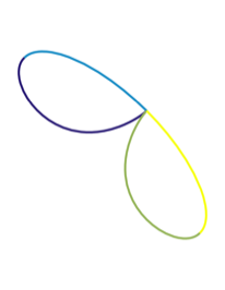
Tropical Decomposition - \(\mathbb{C}\)

Now that we have the NID in 'witness_data', we can compute the tropical decomposition of the component.

To do so, we simply create a 'tropical_curve' object in Matlab. The constructor for this class, provided in this code, performs the decomposition. There are options you can pass in, such as whether you want the complex or real curve, and several numerical tolerances.

For now, let's stick to default mode, which does the decomposition of the complex curve. Here's what I get on my machine:

The curve decomposes on my system fairly rapidly, in about 5 seconds or less. The last command I run is T.ray_sum, checking the balancing condition for this decomposition. The weighted rays of a tropical curve balance to 0, but these balance to -4. What's up with that?

The curve is still homogenized, which I did manually when preparing the system. So instead of balancing to 0, they sum to the negative of the degree of the component, in this case four. Dehomogenizing T and calling ray_sum properly balances.

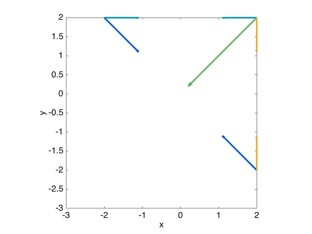
Tropical Decomposition - \(\mathbb{R}\)

Now we will decompose the real part.

This time, we let S be the real decomposition. We compute it, and the dehomogenize. The rays are a subset of the complex set of rays. Notice that the ray_sum does not equal the zero vector! This is because some complex intersections are not real, and have no real paths leading through them. Hence, the real decomposition does not balance.

To conclude, I present S.arrange()